tl;dr – Use .groupby and .transform to achieve SQL-like window functionality in Pandas
Slicing and dicing data using Pandas and SQL is a key skillset for any Data Scientist.
Data Scientists will typically work with both SQL and Pandas for transforming data depending on the specific use case and where the data is stored. For example, SQL is typically used when working directly with data in a database i.e. creating new tables or views of the data. Pandas is used more often when preprocessing data for machine learning or visualisation workflows.
It is important to be fluent with both SQL and Pandas syntax to be able to seamlessly transform your data for the business question you are trying to answer.
However, there are cases where carrying out certain transformations are easier to express in one language than the other.
For me, this seems to always happen when trying to carry out transformations involving Window Functions using Pandas. I don’t know what it is, but I find the SQL syntax for window functions to be much more intuitive.
In this post, I will describe the differences between SQL and Pandas syntax for applying window function calculations to different partitions of your data.
What is a Window Function?
“A window function performs a calculation across a set of table rows that are somehow related to the current row.” Postgres documentation
Window functions allow users to perform aggregations and calculations against different cross-sections (partitions) of the data. In contrast to standard aggregation functions (e.g. sum, mean, count etc.) which return a single value for each partition defined in the query, window functions return a value for each row in the original table.
When would you use a Window Function?
I find there are two main scenarios in the Data Science workflow that involve window functions:
- interpolating or imputing missing values based on statistical properties of other values in the same group
- creating new features for ML models
When you have panel data , window functions are useful for augmenting your dataset with new features that represent aggregate properties of specific partitions within your data.
For example, imagine you are creating a model to predict the price of houses in your neighbourhood given various information about each house such as the house type (e.g. detached, apartment etc.), floor area, number of bedrooms, number of bathrooms etc.
One feature you might want to create for your model is to compare the floor area of the current house to the median area for a house of that specific type. The hypothesis being: if the house has a larger floor area than the median area for a comparable house type, then it is more likely to be priced at the top end of the market.
In order to calculate this feature we would need to create a new column that, for each row, contains the median house price for the current row’s house type. We could then calculate the difference between the house’s area and its group median to use as a feature in our model.
This new feature would require a window function that would calculate and return a value for each row in the dataset with the median house price of that group.
Window Functions in SQL
The Postgres database documentation has a great tutorial on window functions.
Here is a quick recap.
To form a window function in SQL you need three parts:
- an aggregation function or calculation to apply to the target column (e.g.
SUM(),RANK()) - the
OVER()keyword to initiate the window function - the
PARTITION BYkeyword which defines which data partition(s) to apply the aggregation function - (optional) the
ORDER BYkeyword to define the required sorting within each data partition. For example, if the order of the rows affects the value of the calculation
Window Functions in Pandas
.groupby is the basis of window functions in Pandas
I think my confusion when trying to translate SQL window functions to Pandas stems from the fact that you don’t explicitly use the GROUP BY keyword for window functions in SQL. Whereas, in Pandas, the basis of window functions is the .groupby
function.
.groupby in Pandas is analogous to the PARTITION BY keyword in SQL. The groupby clause in Pandas defines which partitions (groups) in the data the aggregation function should be applied to.
.transform allows you to apply complex transformations
In addition to specifying the data partitions using .groupby, we need to define which aggregation or calculation to apply to the data partitions. This can be achieved using the .transform
function.
The .transform function takes a function (i.e. the function which calculates the desired quantity) as an argument and returns a dataframe with the same length as the original.
The function supplied to .transform can either be a string (for simple aggregation functions like ‘sum’, ‘mean’, ‘count’) or a callable function (i.e. lambda function
) for more complex operations.
You don’t always have to use .transform
If the function you are applying to your data is not an aggregation function, i.e. it naturally returns a value (row) for every row in the dataframe, rather than a single row, you don’t need to use the .transform keyword.
For example, if you want to create a new column with the values within each group shifted by one (i.e. in a timeseries, the previous day’s value) you can omit the .transform function and simply use the builtin Pandas function instead – in this case the .shift() function. This is because shifting the data naturally returns a value for each row, rather than a single aggregated value for the group.
Examples
The best way to explain the differences is by demonstrating with some examples.
For this window functions demo we will use a timeseries dataset of stock prices for various companies. The code below shows some simple setup for collecting this data.
💻 There is an accompanying notebook for this blog post available in the Engineering For Data Science GitHub repo if you want to try out the examples yourself.
Setup
Install requirements if necessary
# install required libraries if necessary
pip install matplotlib pandas ffn
Import Libraries
import datetime
import random

import ffn
import matplotlib.pyplot as plt

import pandas as pd

%matplotlib inline
Collect Data
We will use one of my favourite libraries for financial analysis – the ffn library – to collect the data in one line of code.
tickers = [
"AAPL", # apple
"DIS", # disney
"NKE", # nike
"TSLA", # tesla
]
# get stock price data
prices = ffn.get(tickers, start="2018-01-01")
# convert data into 'long' table format for purposes of this exercise
prices = prices.melt(ignore_index=False, var_name="ticker", value_name="closing_price")
# reset index to make 'Date' a column
prices = prices.reset_index()
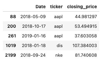
# display 5 example rows in the dataset
prices.sample(5).sort_index()
Save to SQLite Database
In order to demonstrate and compare the SQL syntax to Pandas we will save this data in a simple in-memory SQLite database. This allows us to use directly SQL syntax to read and transform the data.
import sqlite3

# create connection to in memory sqlite db
with sqlite3.connect(":memory:") as conn:

    # save prices dataframe to sqlite db
    prices.to_sql(name="prices", con=conn, index=False)
Let’s take some examples using the stock prices dataset to compare the differences between window functions in SQL and the equivalent in Pandas.
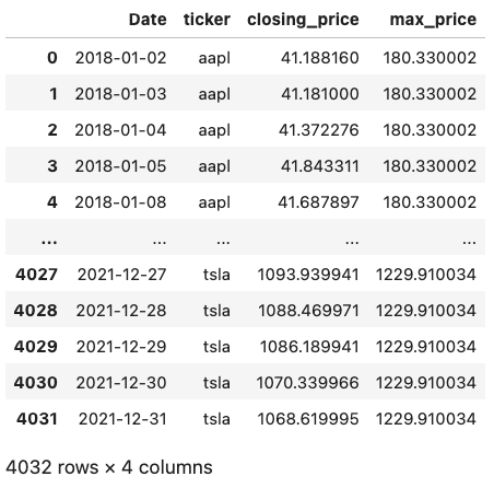
Example 1: Calculating the maximum stock price for each company in the time period
SQL
We calculate the maximum stock price for each ticker by using the MAX function in conjunction with a window function:
- the window function is initiated with the
OVERkeyword - we specify that the
tickercolumn should be used to partition the data
This will return a table of the same length as the original, but with a new column called max_price that contains the maximum stock price the relevant company during time period the data covers.
ex1_sql_query = """
SELECT
    date(Date) as Date
    , ticker
    , closing_price
    , MAX(closing_price) OVER(PARTITION BY ticker) as max_price
FROM
    prices
"""
# use pandas read_sql to execute the query and return a dataframe
ex1_sql = pd.read_sql(ex1_sql_query, con=conn)
ex1_sql
Pandas
We use the groupby function to partition the data by ticker and provide max to the transform function to get a new column which shows the maximum share price for that ticker.
Note that as max is a simple aggregation function, we can simply pass it as a string to the transform function instead of providing a new function (e.g. lambda function).
# copy dataframe to avoid overwritting original (optional)
ex1_pandas = prices.copy()

# add new column
ex1_pandas["max_price"] = ex1_pandas.groupby("ticker")["closing_price"].transform("max")

ex1_pandas
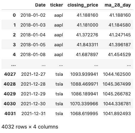
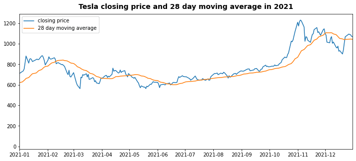
Example 2: 28 day closing price moving average for each company
SQL
When calculating a moving average, the order of values within the group are important (they should be in chronological order), therefore we need to order the values within the group by the date.
Additionally, in SQL, to define the rolling window we specify that the average should be calculated using the preceding 27 rows and the current row (28 in total).
ex2_sql_query = """
SELECT
    date(Date) AS Date
    , ticker
    , closing_price
    , AVG(closing_price) OVER(
        PARTITION BY ticker
        ORDER BY date(Date)
        ROWS BETWEEN 27 PRECEDING AND CURRENT ROW
    )
     AS ma_28_day
FROM
    prices
"""
ex2_sql = pd.read_sql(ex2_sql_query, con=conn)
ex2_sql
Pandas
To achieve the same in Pandas we can create a new column in the dataframe (‘ma_28_day’) using groupby and transform. We utilise Python’s lambda syntax
to define what function should be applied to each group. In this case we want to use calculate the average (mean) over a 28 row rolling window.
Remember to sort the Pandas dataframe before applying the window function when using calculations which are sensitive to the ordering of rows
# copy original dataframe (optional)
ex2_pandas = prices.copy()

# add new column
ex2_pandas["ma_28_day"] = (
    ex2_pandas.sort_values("Date")
    .groupby("ticker")["closing_price"]
    .transform(lambda x: x.rolling(28, min_periods=1).mean())
)

ex2_pandas
Example 3: Get previous day’s closing share price for each ticker
SQL
ex3_sql_query = """
SELECT
    date(Date) AS Date
    , ticker
    , closing_price
    , LAG(closing_price, 1) OVER(
        PARTITION BY ticker
        ORDER BY date(Date)
    ) AS previous_close
FROM
    prices
"""
ex3_sql = pd.read_sql(ex3_sql_query, con=conn)
ex3_sql
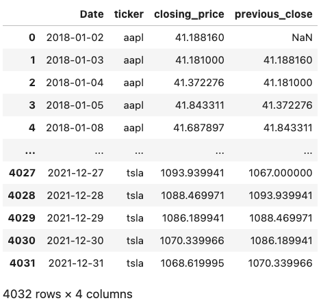
Pandas
In this example, we don’t need to use the transform function because shift naturally returns a value for each row in the data, rather than an aggregation.
ex3_pandas = prices.copy()

ex3_pandas["previous_close"] = (
    ex3_pandas.sort_values("Date").groupby("ticker")["closing_price"].shift(1)
)

ex3_pandas
Example 4: Daily Percentage Return
SQL
In order to calculate the daily return we need to calculate the previous close in a subquery (or CTE) and then use that value to calculate the percentage change increase or daily return.
ex4_sql_query = """
SELECT
    Date
    , ticker
    , closing_price
    , closing_price/previous_close - 1 AS daily_return
FROM
    (
    SELECT
         date(Date) AS Date
        , ticker
        , closing_price
        , LAG(closing_price,1) OVER(
            PARTITION BY ticker ORDER BY date(Date)
        ) AS previous_close
    FROM
        prices
)
"""
ex4_sql = pd.read_sql(ex4_sql_query, con=conn)
ex4_sql
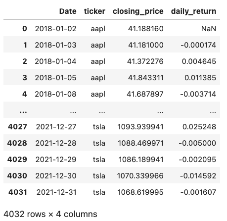
Pandas
Here we can use the lambda function syntax to apply a more complex calculation to each group.
ex4_pandas = prices.copy()

ex4_pandas["daily_return"] = (
    ex4_pandas.sort_values("Date")
    .groupby("ticker")["closing_price"]
    .transform(lambda x: x / x.shift(1) - 1)
)

ex4_pandas
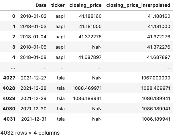
Example 5: Missing Data Interpolation
Pandas
For last this example we will just use Pandas to demonstrate how to use window type functions to interpolate missing data.
First we randomly remove some data to simulate missing data in a real world dataset.
We can then use interpolation or imputation functions to fill in the gaps within each group with a quantity that makes the most sense for the situation. For our use case we will use the ‘forward fill’ method to impute the value of the previous closing price if the data is missing.
# copy orginal dataframe
ex5_pandas = prices.copy()

# remove 30% of data randomly
pct_missing = 0.3
num_missing = int(pct_missing * len(ex5_pandas))
indexes = random.sample(range(len(ex5_pandas)), k=num_missing)
mask = [i in indexes for i in range(len(ex5_pandas))]

# mask the dataframe with some random NaNs
ex5_pandas["closing_price"] = ex5_pandas["closing_price"].mask(mask)
# interpolate missing data paritioned by ticker
ex5_pandas["closing_price_interpolated"] = (
    ex5_pandas.sort_values("Date")
    .groupby("ticker")["closing_price"]
    .transform(lambda x: x.interpolate(method="ffill"))
)

ex5_pandas
# verify there is no missing data in the new column
ex5_pandas.isnull().sum()
Date                             0
ticker                           0
closing_price                 1209
closing_price_interpolated       0
dtype: int64
Conclusion
It is an important skill as a data scientist to be flexible enough to be able to carry out data transformation in either SQL or Pandas when completing data analysis.
Sometimes it is easier in one language than another to express the data transformation you want, but it is important to understand how common data transformations, such as window functions, can be achieved in either language.
The transform function in Pandas can be used to achieve SQL window function like transformations on Pandas dataframes and is a great addition to your tool box.
Happy coding!
💻 Link to the accompanying notebook on Github
Further Reading
- Matplotlib: Plotting Subplots in a Loop
- Five Tips to Elevate the Readability of your Python Code
- Do Programmers Need to be able to Type Fast?
- Event Driven Data Validation with Goolge Cloud Functions and Great Expectations
- How to Manage Multiple Git Accounts on the Same Machine
- Gitmoji: Add Emojis to Your Git Commit Messages!